Cascaded current and speed control
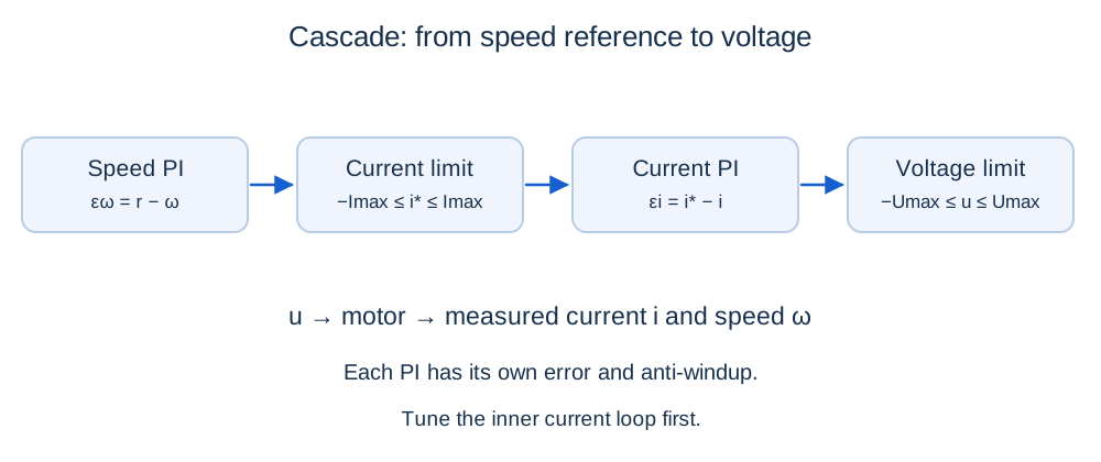
Tune an inner current PI loop, then an outer speed loop with explicit limits.
Before you begin: PI control, converters and transfer functions.
After this lesson you can: tune two loops, compensate back EMF and assess current and voltage feasibility.
Work through the explanation, examples, practical experiment and independent exercises.
Why use an inner loop?
The outer speed controller requests current i*, and the inner controller selects voltage to achieve it. Limiting the current reference helps manage torque. Outer gains are now in A/(rad/s) and A/rad, not the voltage units of lesson 10. Current and speed sensors also have different bandwidth requirements.
Tune current first
Kii/Kpi = R/L; Kpi = L/τi; Kii = R/τi
I/I* = 1/(τi s + 1)
On the fast electrical interval, speed is approximately constant and back EMF is a disturbance. With τi = 0.005 s, L = 0.02 H and R = 2 Ω, Kpi = 4 V/A and Kii = 400 V/(A·s). Ideal 2% settling time is 0.01956 s. Exact cancellation assumes correct parameters and no delay or saturation; it does not eliminate stored magnetic energy. Check heating-induced R changes and converter/sensor bandwidth.
Back-EMF compensation and voltage headroom
u = clip(uraw,−Umax,Umax)
i′ = (u − Ri − keω)/L
Accurate feedforward removes much of the disturbance before integral action reacts. At 60 rad/s and 3 A, the static requirement is 12 V. A 12 V bus has no headroom for a positive current slope. A 24 V bus provides 12 V headroom, allowing up to 600 A/s in this state. Higher gains cannot create voltage headroom.
Tune the outer loop
If the current loop is much faster, approximate i ≈ i*. With ζ = 0.8, ωn = 10 rad/s and base parameters, Kpω = 0.3 A·s/rad and Kiω = 2 A/rad. The inner rate 1/τi = 200 rad/s is substantially faster. Finite current-loop dynamics give:
(J + bτi)(b + ktKpω) > Jτi ktKiω
Besides positive coefficients, the cubic inequality must hold. You cannot accelerate the outer loop indefinitely while keeping the inner loop unchanged.
Two limits and two integrators
vω′ = Kiω(r − ω) + (i* − iraw)/Ttω
vi′ = Kii(i* − i) + (u − uraw)/Tti
Each integrator needs anti-windup at its own limiter. If voltage prevents the inner loop from realizing i* for a long time, outer anti-windup based only on its current-reference limit may be insufficient; track realizable current or condition integration on inner-loop saturation. Limiting i* does not guarantee every actual current sample stays within Imax. Check overshoot, delay and initial conditions. The states vω and vi are in amperes and volts respectively.
Further reading: Imperix: PI control implementations. Notation may differ from this course.
Independent exercises
1. Tune current PI for τi = 0.01 s and find ideal 2% settling time.
Show solution
Kpi = 2 V/A, Kii = 200 V/(A·s), settling time ≈ 0.03912 s.
2. Are 80 rad/s at ML = 0.2 N·m feasible with Imax = 3 A and Umax = 24 V?
Show solution
Required current is 3.6 A, exceeding the limit. Required voltage 15.2 V is available, but current still makes the operating point infeasible. At 3 A, equilibrium speed is 50 rad/s.
Practical work
Implement [i, ω, vi, vω], limits ±24 V and ±3 A, Tti = 0.005 s and Ttω = 0.05 s. Start at zero with a 60 rad/s reference; apply 0.1 N·m at 1 s. Plot i*, i, u, ω and both integrators. Retune the inner loop for τi = 0.05 s, then separately raise R by 20% without retuning. Distinguish bandwidth, mismatch and saturation effects.
Key takeaways
The outer controller requests current and the inner controller requests voltage. Tune inside out and validate both saturated loops together.
Progress is stored only in this browser.