PWM conversion and current ripple
Duty ratio, averaged and switched models, current ripple and additional losses.
Before you begin: RL circuits, back EMF and energy balance.
After this lesson you can: derive average PWM voltage, estimate ripple and test the limits of averaging.
Work through the explanation, examples, practical experiment and independent exercises.
Specify the switching circuit first
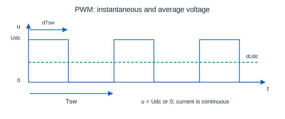
Consider an ideal one-quadrant buck converter with a freewheel diode. When the switch is on, u = Udc; when off with continuous positive current, u = 0. Duty ratio d = ton/Tsw lies between 0 and 1 and switching frequency is 1/Tsw. The diode provides the inductive-current path. This circuit cannot command negative average voltage or sustain reverse diode current; reversal needs another topology.
The averaged equations
Lī′ = dUdc − Rī − keω
Jω′ = ktī − bω − ML
Averaging assumes current and speed change little in a switching period. Compare Tsw with electrical and mechanical time scales and check relative ripple. At low current the diode may stop conducting early, requiring a third zero-current interval. At 60 rad/s and 0.1 N·m, the base motor needs ī = 2.2 A and ū = 10.4 V; with Udc = 24 V, d = 0.4333.
Ripple from the two slopes
Δipp ≈ Udc d(1 − d)/(Lf sw)
Use nearly constant Ri and e during one steady period. The subscript pp means peak-to-peak, not amplitude about the mean. Ripple is largest at d = 0.5. With 24 V, 0.02 H and 2 kHz, the maximum is about 0.15 A; at d = 0.4333 it is 0.14733 A. A rough continuous-current check is ī > Δipp/2. Negative triangular current is not allowed in this diode circuit.
Exact period at fixed speed
a = exp(−dTsw/τ); c = exp[−(1 − d)Tsw/τ]
imax = Ion + (imin − Ion)a
imin = Ioff + (imax − Ioff)c
imin = [Ioff(1 − c) + cIon(1 − a)]/(1 − ac)
Periodicity equates the final current to the initial current. These exponential pieces include changing resistive drop and are valid while current stays positive. Their result approaches the triangular approximation as Tsw/τ becomes small.
Torque, heating and topology
Irms² ≈ ī² + Δipp²/12
PCu ≈ Rī² + RΔipp²/12
Inertia smooths speed but does not remove ripple heating. With R = 2 Ω and Δipp = 0.14733 A, extra copper loss is about 0.00362 W. Reducing L tenfold increases ripple and may invalidate the assumptions. Switch, diode and magnetic losses are excluded.
A bipolar H-bridge switches between +Udc and −Udc, giving average (2d − 1)Udc, not dUdc. Real bridge dead time adds current-direction-dependent error absent from the ideal model.
Independent exercises
1. At Udc = 24 V, L = 0.02 H and d = 0.5, find the minimum frequency for Δipp ≤ 0.1 A.
Show solution
f sw ≥ 3000 Hz, using the continuous-current triangular estimate.
2. Which duty ratio produces −6 V from a 24 V bipolar bridge, and what does that ratio produce in the buck circuit?
Show solution
d = 0.375. The bipolar bridge gives −6 V, while the buck gives +9 V.
Practical work
Plot three steady periods using exact exponentials at 0.5, 2 and 8 kHz. Compare ripple with the approximation. Lower average current until continuous conduction fails. For startup integration, split at PWM edges. Separate averaging error from numerical error and explain why equal average speed does not imply equal losses.
Key takeaways
Average voltage captures slow motion, not ripple or all losses. Formulas depend on topology and conduction mode. PWM period, solver step and control period are different quantities.
Progress is stored only in this browser.