Identifying motor parameters
Estimate resistance, inductance, back-EMF constant, inertia and friction from measurements.
Before you begin: the motor model, exponential responses and linear algebra.
After this lesson you can: design informative experiments and distinguish parameter error from missing physics.
Work through the explanation, examples, practical experiment and independent exercises.
What does identifying parameters mean?
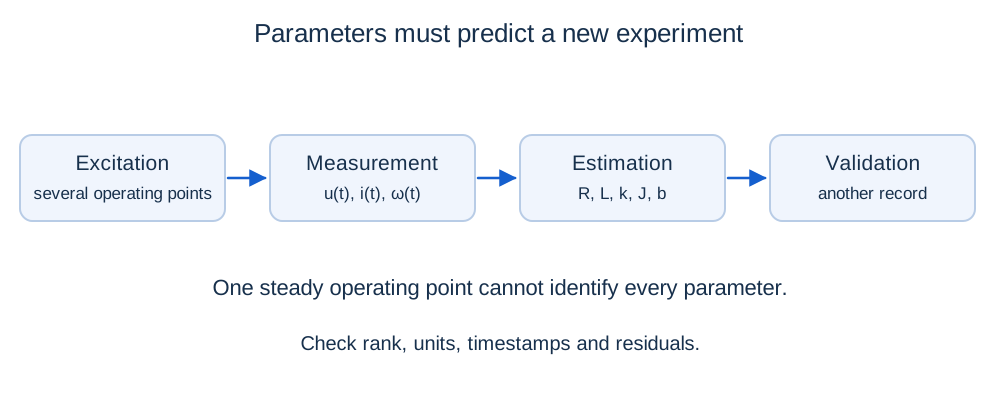
Identification estimates model parameters from inputs and measured outputs. A nameplate may omit parameters or describe a different temperature or assembly. Choose the model structure before fitting numbers. Missing dry friction may be absorbed into fitted b and J, but those values can fail on another experiment. Measure u, i and ω, and know or eliminate load torque.
Resistance and inductance
τe = −t/ln[(I∞ − i(t))/(I∞ − i₀)]
L = Rτe
A stationary rotor removes rotational EMF. With U = 4 V, i₀ = 0, I∞ = 2 A and i(10 ms) = 1.26424 A, obtain R = 2 Ω and L = 0.02 H. One steady point cannot determine L. On a physical test rig, use designed rotor restraint and current limits. Fit several voltage levels to U = RI + Ubrush for one current direction: a significant brush drop makes U/I a biased resistance estimate.
EMF constant, inertia and friction
ln|ω(t)/ω₀| = −(b/J)t
kti − ML = Jω′ + bω
At U = 12 V, I = 2 A and ω = 80 rad/s, ke = 0.1 V·s/rad. Ideal SI consistency gives kt = ke. A zero-current, no-load coast-down identifies only b/J, not both separately. An independent known-torque experiment is needed. At ω = 0, i = 1 A, ML = 0 and acceleration 50 rad/s², J = 0.002 kg·m²; a 1 s coast-down time then gives b = 0.002 N·m·s/rad, assuming no dry friction.
Integral regression instead of noisy derivatives
Y = Φθ; θ = [R,L,ke]ᵀ
θ̂ = arg min ‖Φθ − Y‖²
Each time window supplies one linear equation. Φ needs full column rank. At rest its speed column vanishes, preventing identification of ke; at steady current the increment column vanishes, preventing identification of L. Use informative excitation and adequate recording frequency. Solve with QR/SVD, for example numpy.linalg.lstsq, rather than explicitly inverting ΦᵀΦ. Scale columns. Noise also affects Φ, so ordinary least squares need not be unbiased.
Fitting several points
α̂ = −Σ(tj ln qj)/Σtj²; L̂ = R/α̂
At 5, 10, 15 and 20 ms, synthetic currents 0.78694, 1.26424, 1.55374 and 1.72933 A for 4 V yield L ≈ 0.02000 H. Points close to I∞ make the logarithm sensitive to noise. Fitting the original current exponential is often preferable with noisy data; logarithmic fitting weights errors differently.
Independent validation
Fit one record, then predict another voltage or load step without refitting. Plot measured-minus-model current and speed residuals. Persistent bias and repeatable shapes matter more than one average error. Sensor time shifts can resemble larger L; encoder scale error can resemble different ke. Check timestamps, units and directions before fitting. Negative passive R, L or J estimates call for investigation.
Independent exercises
1. At rest, U = 6 V, I∞ = 3 A and i₀ = 0. At 8 ms current is 1.89636 A. Find R and L.
Show solution
R = 2 Ω. The remaining fraction is 0.36788, so τ ≈ 8 ms and L ≈ 0.016 H.
2. Coast-down reduces speed from 100 to 60.653 rad/s in 0.5 s. Can it identify J and b separately? Find b if J = 0.003 kg·m².
Show solution
Only b/J ≈ 1 s⁻¹ is identifiable. With the independently known J, b ≈ 0.003 N·m·s/rad.
Practical work
Generate an RL response and add 0.01 A standard-deviation current noise using a fixed seed. Compare single-point and all-point estimates over 50 noise realizations. Add a 0.03 A sensor offset and distinguish bias from random scatter. State which parameters each experiment identifies and which record validates the model.
Key takeaways
Parameters require informative data. Validation on another operating condition is essential; fitting the training experiment is not enough.
Progress is stored only in this browser.